The Gray-Scott Model of Autocatalytic Reactions

An autocatalytic reaction, first conceived by the chemist Wilhelm Ostwald in the late 19th century, is a self-sustaining chemical reaction. In its simplest form we have a chemical reaction of the form \(A + X \rightarrow 2X \) where \(X\) is an "autocatalyst particle" and \(A\) is a "resource". This equation seems to imply that the rate at which \(X\) particles are formed increases with time, since it's rate of production would depend on the concentration of \(X\) particles. Indeed, Ostwald himself defined an autocatalytic reaction as one that "shows an acceleration of the rate as a function of time."

Consider the following reaction $$ A + B \rightarrow 2B $$ The law of mass action implies that the rate of the reaction is given by $$ \frac{d\left[B\right]}{dt} = O(\left[A\right]\left[B\right]) = k\left[A\right]\left[B\right] $$ assuming that \(A+B\rightarrow 2B\) is an elementary reaction. The constant \(k\) is called the reaction rate constant.

The \(A\) molecules are lost as they react with the \(B\) molecules. In particular, $$ \frac{d\left[A\right]}{dt} = -k\left[A\right]\left[B\right] $$

Let's assume that the molecules undergo diffusion, moving from regions of high to low concentration according to Fick's law: $$ \frac{\partial\left[B\right]}{\partial t} = k\left[A\right]\left[B\right] + D\nabla^2\left[B\right] $$ where \(D\) is a diffusion constant.

It may be the case that some amount of \(B\) decays over time resulting in a product that no longer reacts with \(A\) (an inert product). In this case we have the stoichiometric equations $$ \begin{align} A+B\rightarrow 2B\\ B\rightarrow\text{inert} \end{align} $$ We'll assume the first equation has a reaction rate \(k_1\), while the second equation has reaction rate \(k_2\left[B\right]\). Hence $$ \begin{align} \frac{\partial\left[B\right]}{\partial t} = k_1\left[A\right]\left[B\right] + D_B\nabla^2\left[B\right] - k_2\left[B\right] \\ \frac{\partial\left[A\right]}{\partial t} = -k_1\left[A\right]\left[B\right] + D_A\nabla^2\left[A\right] \end{align} $$

Now for the final complication: suppose that reactant \(A\) is readded to the system according to some rule, e.g. \(k_f(1-\left[A\right])\) supposing the concentration of A (and B) lie within \([0,1]\). In this case, when the concentration is low \(1-\left[A\right]\) is high, etc. The constant \(k_f\) controls the rate by which \(A\) is fed into the system.

The equations now look like $$ \begin{align} \frac{\partial\left[B\right]}{\partial t} = k_1\left[A\right]\left[B\right] + D_B\nabla^2\left[B\right] - k_2\left[B\right] \\ \frac{\partial\left[A\right]}{\partial t} = k_f(1-\left[A\right]) - k_1\left[A\right]\left[B\right] + D_A\nabla^2\left[A\right] \end{align} $$

Higher-Order Models

Autocatalytic reactions of the form \(A + B \rightarrow B\) are called quadratic or simple [1]. Alternately there is the cubic form $$ A + 2B \rightarrow 3B $$ and, more generally, $$ A + nB \rightarrow (n+1)B. $$ The rate of reaction is \( k\left[A\right]\left[B\right]^n \) for \(n\geq 1\).

Skipping the tedious algebra, we have the follow reaction-diffusion equation for the quadratic form of the Gray-Scott model: $$ \begin{align} \frac{\partial\left[B\right]}{\partial t} = k_1\left[A\right]\left[B\right]^2 + D_B\nabla^2\left[B\right] - k_2\left[B\right] \\ \frac{\partial\left[A\right]}{\partial t} = k_f(1-\left[A\right]) - k_1\left[A\right]\left[B\right]^2 + D_A\nabla^2\left[A\right] \end{align} $$

Pearson's Variation

The paper [2] presents a variant where both reactants are subject to a "non-equilibrium constraint [...] represented by a feed term for" \(A\). We have the stoichiometric equations $$ \begin{align} A + 2B \rightarrow 3B\\ B \rightarrow \text{inert} \end{align} $$

Suppose that the molecules \(A\) and \(B\) are diffusing at rates \(D_A\nabla^2A\) and \(D_B\nabla^2B\) respectively. Furthermore we assume that \(A\) is fed into the system at a rate \(f(1-A)\) and that \(B\) is drained from the system at a rate \(fB\).

Finally, suppose the first reaction proceeds at a rate \(k_1AB^2\) and suppose the second one proceeds at a rate \(k_2B\). Then the resulting reaction-diffusion equations are $$ \begin{align} \frac{\partial\left[B\right]}{\partial t} = k_1\left[A\right]\left[B\right]^2 + D_B\nabla^2\left[B\right] - (f+k_2)\left[B\right]\\ \frac{\partial\left[A\right]}{\partial t} = D_A\nabla^2\left[A\right] - k_1\left[A\right]\left[B\right]^2 + f(1-\left[A\right]) \end{align} $$

Simulation

We can simulate this model easily in Python. The state update function looks like

D_A, D_B, f, k_1, k_2 = 0.16, 0.08, 0.035, 1.0, 0.065
def update(A, B, tmpA, tmpB):
    tmpA[...] = A + D_A * laplacian(A) - k_1 * A * np.square(B) + f * (1.0 - A)
    tmpB[...] = B + D_B * laplacian(B) + k_1 * A * np.square(B) - (f + k_2) * B
    

N = 256
r = 10
A = np.ones((N, N), dtype=np.float32)
B = np.zeros((N, N), dtype=np.float32)
A[N//2 - r:N//2 + r, N//2 - r:N//2 + r] = 0.50
B[N//2 - r:N//2 + r, N//2 - r:N//2 + r] = 0.25
A += 0.01 * np.random.uniform(-1, +1, (N, N))
B += 0.01 * np.random.uniform(-1, +1, (N, N))
tmpA = np.empty_like(A)
tmpB = np.empty_like(B)

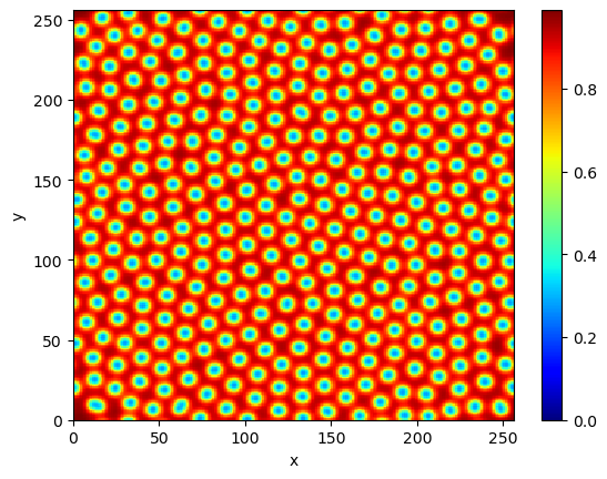
Now we simulate the system and take a picture of A:

for _ in range(200_000):
    update(A, B, tmpA, tmpB)

    grid_swap = A
    A = tmpA
    tmpA = grid_swap

    grid_swap = B
    B = tmpB
    tmpB = grid_swap
plot(A)

Different interesting values for the parameters can be found in chapter 4 of [3]. An interesting further direction would be to simulate the Belousov–Zhabotinsky reaction.

References

1. [0] Schuster, Peter, What is special about autocatalysis?, Monatshefte für Chemie - Chemical Monthly (2019) 150:763-775
2. [1] Gray, P., Scott, S. K., "Autocatalytic Reactions in the Isothermal Continuous Stirred Tank Reactor", Chemical Engineering Science, Vol. 38, No. 1, pp. 29-43, 1983
3. [2] Pearson, John E., "Complex Patterns in a Simple System", Science, Vol. 261, 9 July 1993
4. [3] Rougier, Nicolas P., From Python to Numpy
5. [4] Sebastian Kehl, Sebastian Ohlmann, Klaus Reuter, Python for HPC